Solving the Problem

As you can see, manually creating solutions is a tedious task and requires taking into account each constraint carefully. This is the reason the Dispatcher class was created. This class allow us to just define the order in which operations are sequenced and the machines in which they are processed. The Dispatcher class will take care of the rest.

Let’s see an example of how to use the Dispatcher class to solve the previous instance. In this case, a reasonable solution is to process, for each job, the operations in the order they are defined in the instance. We can do this as follows:

from job_shop_lib import JobShopInstance, Operation

CPU = 0
GPU = 1
DATA_CENTER = 2

job_1 = [Operation(CPU, 1), Operation(GPU, 1), Operation(DATA_CENTER, 7)]
job_2 = [Operation(GPU, 5), Operation(DATA_CENTER, 1), Operation(CPU, 1)]
job_3 = [Operation(DATA_CENTER, 1), Operation(CPU, 3), Operation(GPU, 2)]

jobs = [job_1, job_2, job_3]

instance = JobShopInstance(jobs, name="Example")

from job_shop_lib.dispatching import Dispatcher

dispatcher = Dispatcher(instance)

for i in range(3):
    dispatcher.dispatch(job_1[i], job_1[i].machine_id)
    dispatcher.dispatch(job_2[i], job_2[i].machine_id)
    dispatcher.dispatch(job_3[i], job_3[i].machine_id)

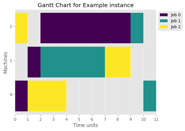
The dispatcher took care of any possible overlaps providing the expected solution, as we can see below

from job_shop_lib.visualization.gantt import plot_gantt_chart
import matplotlib.pyplot as plt

plt.style.use("ggplot")

_ = plot_gantt_chart(dispatcher.schedule)

Even though the dispatcher creates solutions easily, they are crafted manually/procedurally and therefore will usually be far from optimal. It is interesting to introduce solvers that find solutions according to certain optimality criteria.

A solver is any Callable object that takes as input a JobShopInstance class and returns a Schedule with a complete solution of the instance.

In this example, we are going to use the CPSolver class, contained inside job_shop_lib.solvers package, which uses CP-SAT solver from Google OR-Tools.

from job_shop_lib.constraint_programming import ORToolsSolver

solver = ORToolsSolver()
schedule = solver(instance)
schedule.schedule

[[S-Op(operation=O(m=0, d=1, j=0, p=0), start_time=0, machine_id=0),
  S-Op(operation=O(m=0, d=3, j=2, p=1), start_time=1, machine_id=0),
  S-Op(operation=O(m=0, d=1, j=1, p=2), start_time=10, machine_id=0)],
 [S-Op(operation=O(m=1, d=1, j=0, p=1), start_time=1, machine_id=1),
  S-Op(operation=O(m=1, d=5, j=1, p=0), start_time=2, machine_id=1),
  S-Op(operation=O(m=1, d=2, j=2, p=2), start_time=7, machine_id=1)],
 [S-Op(operation=O(m=2, d=1, j=2, p=0), start_time=0, machine_id=2),
  S-Op(operation=O(m=2, d=7, j=0, p=2), start_time=2, machine_id=2),
  S-Op(operation=O(m=2, d=1, j=1, p=1), start_time=9, machine_id=2)]]

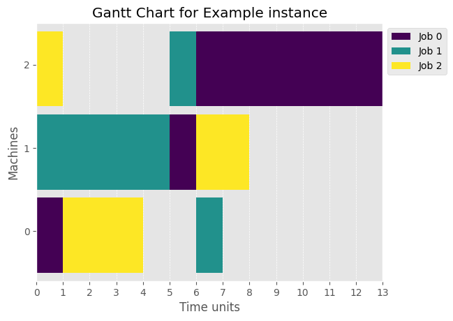
This class returns a Schedule object with a complete solution of the instance. It also incorporates some metadata of the solution, such as the time it took to solve the instance and the status of the solution:

print(f"Is complete?: {schedule.is_complete()}")
print(f"Meta data: {schedule.metadata}")
print(f"Makespan: {schedule.makespan()}")

Is complete?: True
Meta data: {'status': 'optimal', 'elapsed_time': 0.027423290999649907, 'makespan': 11, 'solved_by': 'ORToolsSolver'}
Makespan: 11

We can now plot the gantt chart of the solution provided by the solver which is not only valid and complete, but clearly better in terms of makespan.

_ = plot_gantt_chart(schedule)